Loading pre-trained models
[1]:
import matplotlib.pyplot as plt
import numpy as np
import jax
from jax import numpy as jnp

import diffmahnet
[2]:
# View available pre-trained models
available_names = diffmahnet.pretrained_model_names
available_names
[2]:
['satflow_v1_0train.eqx',
 'cenflow_v1_0.eqx',
 'cenflow_v2_0.eqx',
 'satflow_v2_0.eqx',
 'satflow_v1_0.eqx',
 'cenflow_v1_0train.eqx']
[3]:
centrals_model = diffmahnet.load_pretrained_model("cenflow_v2_0.eqx")
satellites_model = diffmahnet.load_pretrained_model("satflow_v2_0.eqx")
Generate diffmah parameters
Condition on a few values of \(u = (\log M_{\rm obs}, t_{\rm obs})\)
For each conditional value, generate a sample of 1000 MAHs
[4]:
n_sample = 1000
m_grid = jnp.array([11.0, 12.5, 14.0])
t_grid = jnp.array([2.0, 7.5, 13.0])
m_vals, t_vals = [jnp.repeat(x.flatten(), n_sample)
                  for x in jnp.meshgrid(m_grid, t_grid)]
print(m_vals)
print(t_vals)
[11. 11. 11. ... 14. 14. 14.]
[ 2.  2.  2. ... 13. 13. 13.]
Create functions roughly equivalent to mc_diffmah_*pop() for our trained models
[5]:
# Note a few differences from mc_diffmah_cenpop:
# - Only returns a single set of DiffmahParams
# - Does not depend on lgt0 or t_peak
mc_diffmahnet_cenpop = centrals_model.make_mc_diffmahnet()
mc_diffmahnet_satpop = satellites_model.make_mc_diffmahnet()

randkey = jax.random.key(0)
keys = jax.random.split(randkey, 2)
cenflow_diffmahparams = mc_diffmahnet_cenpop(
    centrals_model.get_params(), m_vals, t_vals, keys[0])
satflow_diffmahparams = mc_diffmahnet_satpop(
    satellites_model.get_params(), m_vals, t_vals, keys[1])
[6]:
# Plot mass accretion histories from the predicted diffmah parameters
tgrid = jnp.linspace(0.5, t_vals, 100).T
cen_mah = diffmahnet.log_mah_kern(
    cenflow_diffmahparams, tgrid, np.log10(13.8))
sat_mah = diffmahnet.log_mah_kern(
    satflow_diffmahparams, tgrid, np.log10(13.8))
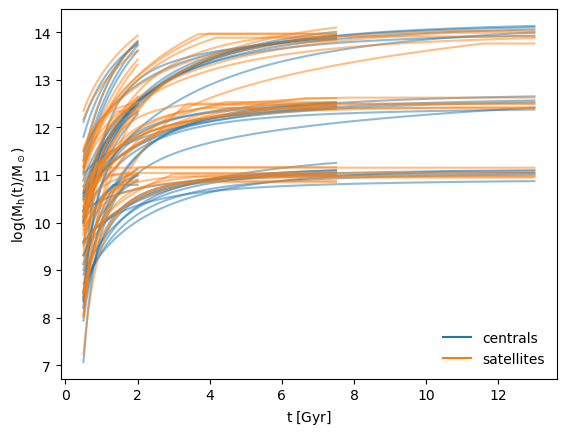
[7]:
# Plot the MAH of every 200th halo (5 per set of {M_obs, t_obs})
plt.plot([], [], label="centrals", color="C0")
plt.plot([], [], label="satellites", color="C1")
plt.plot(tgrid[::200].T, cen_mah[::200].T, color="C0", alpha=0.5)
plt.plot(tgrid[::200].T, sat_mah[::200].T, color="C1", alpha=0.5)
plt.legend(frameon=False)
plt.xlabel("$\\rm t \\; [Gyr]$")
plt.ylabel("$\\rm \\log(M_h(t)/M_\\odot)$")
plt.show()